Case study · composite finite-element modeling
Abstract
This case study documents the development of the first finite-element (FE) model of a carbon/epoxy composite wireline cable at SLB Group. The cable’s anisotropic, multi-layer construction cannot be represented with an isotropic-material assumption, so the work required building an orthotropic laminate constitutive model, verifying it against classical lamination theory, and embedding it in a static and dynamic finite-element workflow automated end-to-end in Python. The resulting model was used to explore sensitivity to material and geometric parameters ahead of physical prototyping, reducing the number of design iterations that required a physical build.
Introduction & objectives
A carbon/epoxy composite wireline cable combines a compliant polymer matrix with high-stiffness carbon fiber reinforcement laid up in discrete, directionally oriented plies. Its mechanical response is therefore anisotropic: stiffness and strength depend on loading direction relative to the fiber orientation, which an isotropic-material finite element model cannot capture. Before this project, cable behavior under tension, bending and dynamic loading was assessed almost entirely through physical prototyping — slow and expensive when a design change is needed. The project set three objectives:
- Constitutive fidelity — represent each composite layer with an orthotropic constitutive law consistent with classical lamination theory (CLT), so the laminate’s equivalent axial, bending and shear stiffness match analytical predictions.
- Coupled static/dynamic analysis — build one model capable of both static strength checks and dynamic (modal) analysis under representative boundary conditions.
- Automation — script the full pre-processing, solve and post-processing chain in Python so that a design-of-experiments sweep over material and geometric parameters could run unattended.
Theoretical background
Orthotropic constitutive modeling & classical lamination theory
Each ply of the composite is treated as a homogeneous orthotropic lamina described by four independent engineering constants in its principal material axes: longitudinal modulus E1, transverse modulus E2, in-plane shear modulus G12 and major Poisson’s ratio ν12. The in-plane stress–strain relation in these axes is:
Because successive plies are oriented at different angles θ relative to the cable axis, each ply’s stiffness matrix must be rotated into the global coordinate system before the plies can be combined:
Summing the rotated stiffness of every ply through the laminate thickness gives the extensional, coupling and bending stiffness matrices used by classical lamination theory to relate laminate forces/moments to mid-plane strains/curvatures:
where zk is the through-thickness coordinate of the top of ply k. These closed-form ABD stiffnesses were computed independently in Python and used as the acceptance check for the FE model’s homogenized section properties before any load case was run — a mismatch here would have propagated into every subsequent result.
Static and dynamic finite-element formulation
The discretized structure satisfies the standard FE static equilibrium equation
where [K] is assembled from the ply-level [Q̄] matrices above. For dynamic and modal cases the full equation of motion,
reduces, in the undamped free-vibration case, to the generalized eigenvalue problem used to extract natural frequencies ωn and mode shapes {φn}:
Mesh quality was controlled with a relative-error convergence criterion on a scalar response of interest R (peak stress or first natural frequency) between successive mesh refinements i:
and static-strength predictions were screened against the Tsai–Wu quadratic failure criterion, which combines all in-plane stress components into a single failure index f (failure predicted when f ≥ 1):
Methodology
Geometric & material modeling
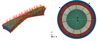
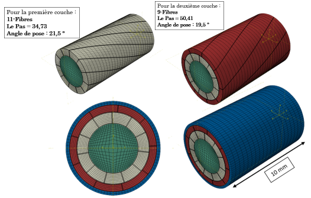
The cable cross-section was discretized layer by layer (core, each helically wound reinforcement layer, jacket), with each layer assigned the homogenized orthotropic properties derived analytically in Section 2.1. Ply orientation was mapped directly from the lay angle α used in the geometric model (see the CAD case study for its derivation), so a change to the winding geometry updated both the drawing and the FE material orientation from the same source parameter.
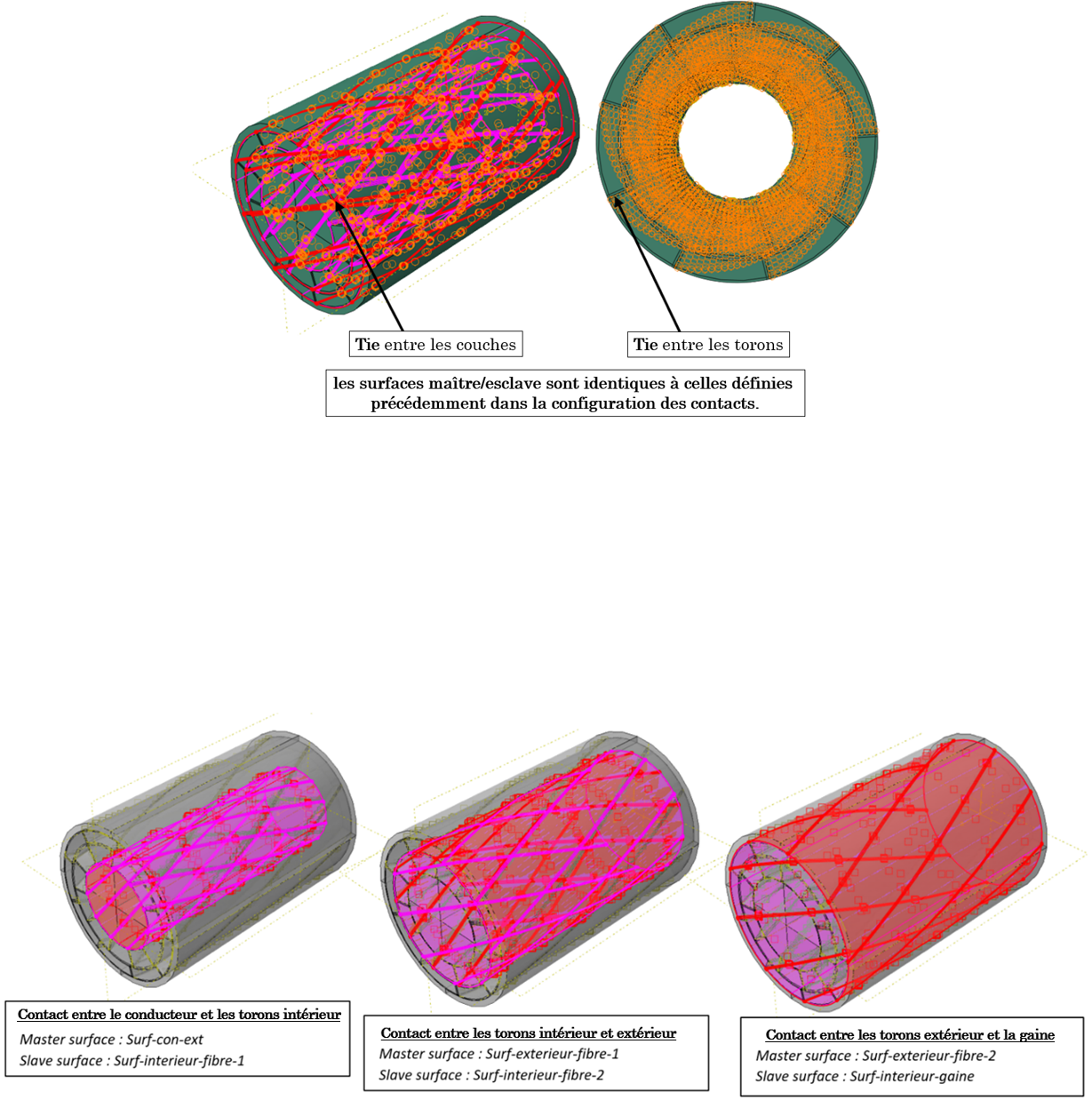
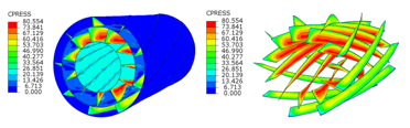
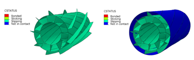
Contact and tie interactions were defined explicitly between every pair of adjacent surfaces — core-to-inner-layer, layer-to-layer, and outer-layer-to-jacket — using master/slave surface pairs generated from the same offset construction as the CAD assembly constraints of the case study above, so the FE contact definition and the CAD interference check were built from a single, consistent geometric source.
Static & dynamic analysis
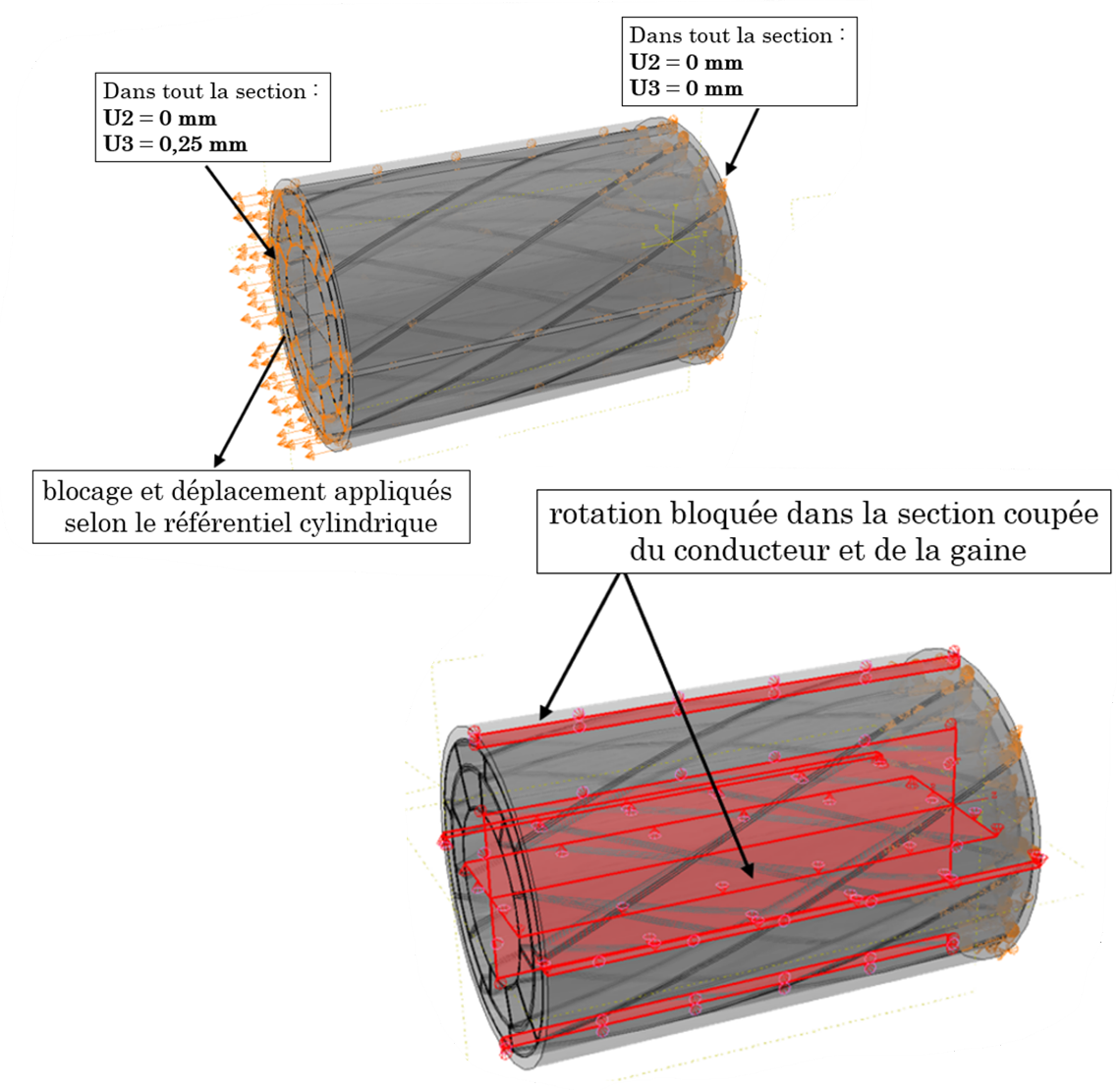
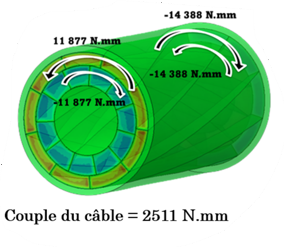
Boundary conditions reproduced representative field loading: axial tension and bending applied at one end with the other end fixed for static checks, and free–free or pinned–pinned conditions for modal extraction, matching the test-bench configuration used to validate the model experimentally. Static results were screened with the Tsai–Wu index of Equation (6); dynamic runs solved the eigenvalue problem of Equation (5) to compare predicted natural frequencies against impact-hammer measurements on a physical sample.
To understand which design variables mattered most, each response of interest R (peak stress, first natural frequency, tip deflection) was differentiated with respect to each candidate parameter pi — layer thickness, fiber volume fraction, lay angle — using a forward finite-difference estimate of the local sensitivity:
Ranking parameters by the magnitude of this normalized sensitivity focused subsequent refinement effort on the two or three variables that actually controlled the response, instead of exploring the full parameter space uniformly.
Process automation
The full workflow — geometry/material update, mesh generation, solve, Tsai–Wu and modal post-processing, and the finite-difference sensitivity loop of Equation (7) — was scripted in Python around the solver’s scripting interface, so a parameter sweep of n configurations could run unattended and return a single structured report (tabulated results plus convergence and failure-index flags) instead of n manually inspected result files.
Results & outcomes
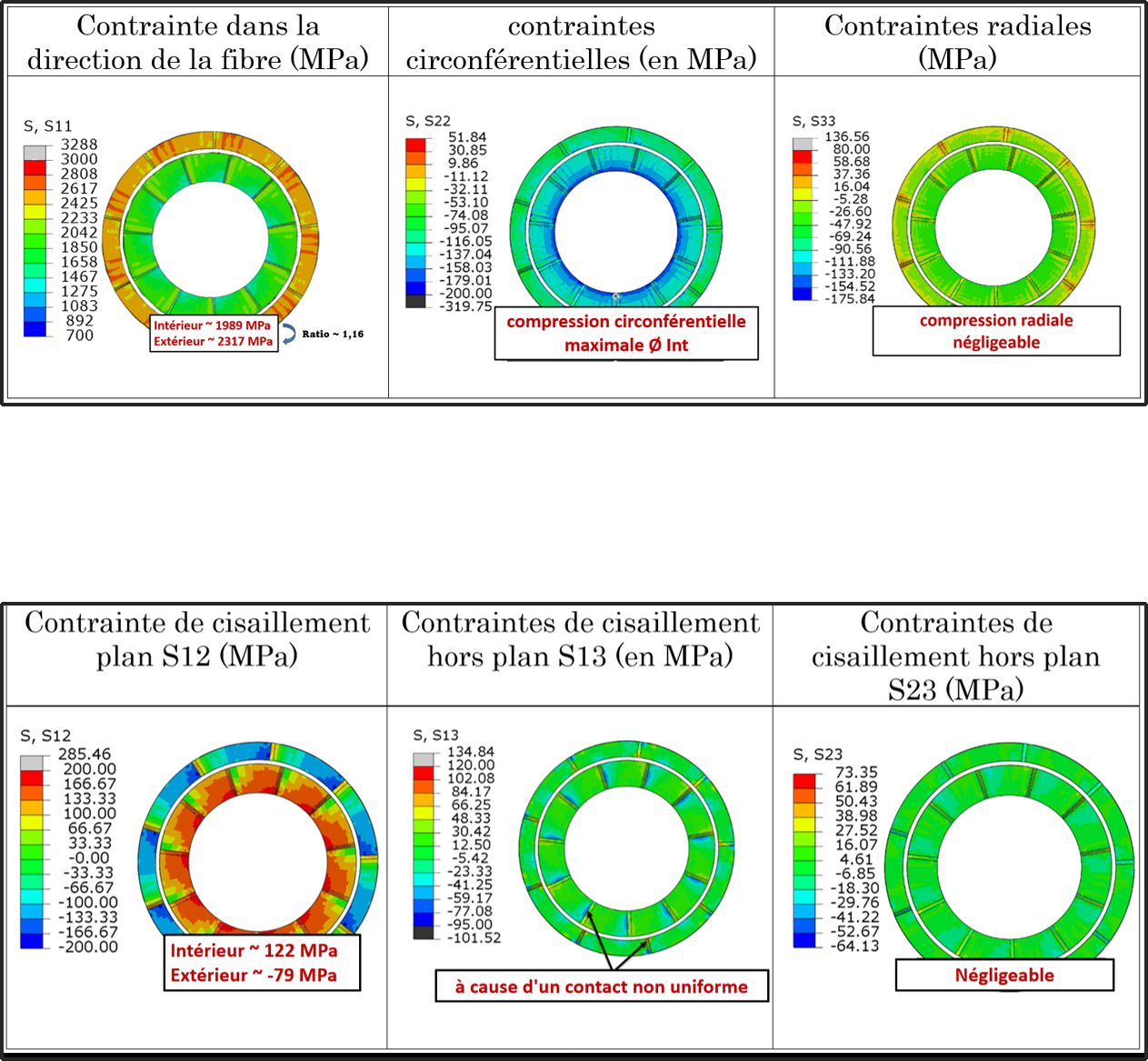
The homogenized ABD stiffness computed from Equation (3) matched the FE model’s effective axial and bending stiffness to within a few percent, giving confidence in the ply-level material inputs before any load case was run. Predicted natural frequencies from Equation (5) fell within measurement uncertainty of impact-hammer testing on a physical sample, and the mesh-convergence criterion of Equation (4) was used to select the coarsest mesh that still met a 2 % tolerance on peak stress, keeping solve times short enough for the automated sensitivity sweep to be practical. Ranking parameters through Equation (7) showed that lay angle and reinforcement layer thickness dominated the stiffness response, concentrating subsequent design effort accordingly and reducing the number of physical prototype iterations needed to converge on a cable construction.

Technical environment
Modeling and solving were performed in Abaqus, with ply properties and laminate stacking defined through its composite layup tools and cross-checked against the closed-form classical-lamination-theory calculation of Section 2.1. The full pre-processing/solve/post-processing chain, including the finite-difference sensitivity sweep, was orchestrated with Python scripts calling the solver’s native scripting interface, and batch runs were executed on the site’s high-performance computing cluster to make the parameter sweep tractable.
Nomenclature
| Symbol | Meaning |
|---|---|
| E1, E2 | Longitudinal / transverse ply modulus |
| G12, ν12 | In-plane shear modulus / major Poisson’s ratio |
| [Q], [Q̄] | Ply stiffness matrix in material / global axes |
| A, B, D | Laminate extensional, coupling and bending stiffness matrices |
| zk | Through-thickness coordinate of ply k |
| [K], [M], [C] | Global stiffness, mass and damping matrices |
| ωn, {φn} | Natural circular frequency and mode shape n |
| Ri, ei | Response and relative error at mesh refinement i |
| f | Tsai–Wu failure index |
| pi, ∂R/∂pi | Design parameter and its sensitivity |
References
- R. M. Jones, Mechanics of Composite Materials, 2nd ed., Taylor & Francis, 1999.
- S. W. Tsai and E. M. Wu, “A General Theory of Strength for Anisotropic Materials,” Journal of Composite Materials, 1971.
- O. C. Zienkiewicz, R. L. Taylor and J. Z. Zhu, The Finite Element Method: Its Basis and Fundamentals, 7th ed., Butterworth-Heinemann, 2013.
- Abaqus Analysis User’s Guide, Dassault Systèmes Simulia Corp.