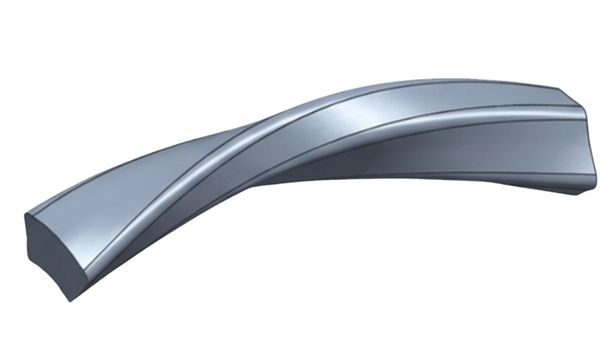
Case study · parametric CAD & dimensional engineering
Abstract
This case study documents the design and technical-documentation workflow developed for the mechanical components of a carbon/epoxy composite wireline cable programme at SLB Group. The central engineering difficulty was representing the true three-dimensional geometry of helically wound reinforcement elements inside a parametric CAD model — rather than approximating it with straight extrusions — so that clearances, developed (cut) lengths and manufacturing drawings would remain dimensionally consistent with the physical part. The resulting master model, driven by a small set of independent geometric parameters and verified through worst-case and statistical tolerance-stack analysis, was translated into ISO-compliant detail drawings and managed under configuration control in Windchill PLM.
Introduction & objectives
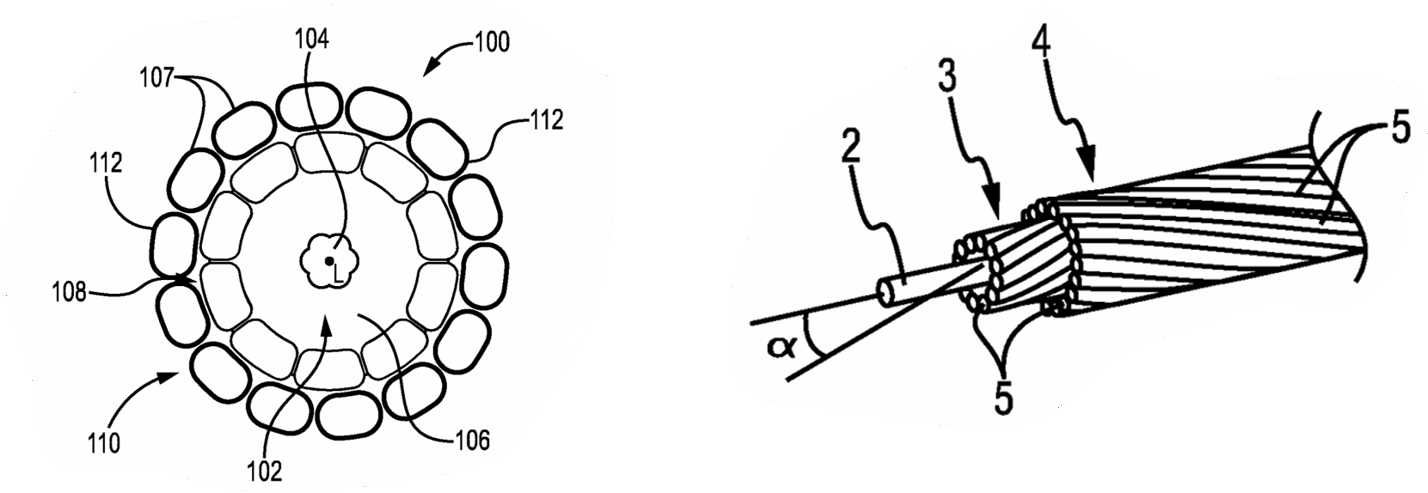
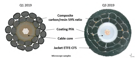
Composite wireline cables are built from a central core, one or more layers of helically wound strength members (carbon and/or steel), and an extruded polymer jacket. Because the strength members follow a helical path rather than a straight one, any CAD representation that ignores the helix angle will misstate the part’s outer envelope, its developed (uncoiled) length, and the clearances between layers — all of which are load-bearing, manufacturing-critical dimensions. The project therefore combined three objectives:
- Parametric geometric fidelity — build a CAD architecture able to represent multi-layer helical cable geometry from a minimal set of independent design parameters (lay length, lay angle, strand diameter, number of strands per layer), so the model regenerates correctly for any construction without being rebuilt from scratch.
- Defensible documentation — produce ISO 128 / ISO 1101–compliant 2D drawings with GD&T callouts sized to the functional requirement of each interface, rather than blanket tolerances.
- Configuration control — manage the resulting CAD data set and its revisions inside Windchill PLM so that R&D, manufacturing and quality could work from a single source of truth.
Sections 2 and 3 below present the geometric and dimensional-tolerancing theory used to meet objective 1 and 2, Section 4 walks through the resulting workflow (mission details), and Section 5 summarizes measurable outcomes.
Theoretical background
Geometric modeling of helically wound strength members
Each strength member follows a right-circular helix wound on a cylinder of pitch radius R. Parametrizing the curve by the winding angle t, its coordinates are:
where p is the lay length (axial advance per full turn) and n is the number of turns spanned by the model. This single relation was entered as a driving equation in the CAD parametric-sketch/curve-from-equation feature, so the strand path updates automatically whenever R or p changes.
The lay angle α — the angle between a strand’s local tangent and the cable axis — follows directly from the pitch and radius:
For a layer built from N strands laid with uniform angular spacing, the angular offset of the k-th strand is:
Equations (1)–(3) were the only geometric drivers needed to regenerate an entire multi-strand layer from four independent inputs (R, p, strand diameter d, and N) — which made evaluating alternative cable constructions a matter of changing four numbers rather than rebuilding geometry.
A second, more subtle issue is orienting the strand’s circular cross-section as it is swept along the helix: a profile held at a fixed orientation will visibly distort near the ends of a sweep. The correct orientation keeps the profile normal to the local tangent vector T(t), obtained by normalizing the derivative of r(t):
so that ∥r′(t)∥ = √(R² + (p/2π)²), a constant — confirming that a helix swept at constant radius and pitch has constant tangent-vector magnitude, which is what allows a CAD sweep feature to use a single, constant normal-to-path orientation rule along the whole curve.
Dimensional tolerancing theory
Two tolerancing questions had to be answered for every interface on the drawings: how tight should an individual tolerance be, and do a chain of individually acceptable tolerances still guarantee the assembly will fit? ISO 286 answers the first question by defining a standard tolerance unit i (in micrometres) as a function of the nominal diameter D (in millimetres, geometric mean of the applicable size range):
Multiplying i by the grade-dependent factor for the chosen IT grade (e.g. IT7, IT9) gives the tolerance band appropriate to the functional role of the feature — tight grades for fitted interfaces (e.g. socket bores), looser grades for non-critical envelope dimensions.
For a stack of n individually toleranced dimensions contributing to one functional gap or clearance, two stack-up models were used depending on criticality. The conservative, worst-case bound sums the absolute contributions:
which guarantees the fit under any combination of tolerances but is often overly strict. Where the individual contributors could reasonably be treated as independent random variables, the statistical (root-sum-square) model was used instead, giving a much more realistic — and less conservative — combined tolerance:
Finally, for position callouts referenced at Maximum Material Condition (MMC), the effective tolerance available on the shop floor increases as the produced feature departs from MMC toward its Least Material Condition, by the bonus tolerance:
This bonus was used deliberately on non-critical fastener and locating features to reduce manufacturing rejection rates without loosening the nominal positional requirement.
Methodology
Analysis & solution selection
Three CAD platforms already present in the wider organization (Creo, SolidWorks, CATIA V5) were evaluated against five weighted criteria: native associativity between 3D model and 2D drawing, quality of equation/relation-driven parametric modeling, native Windchill PLM integration, licence availability within the team, and learning-curve cost. Each candidate j was scored on each criterion i (0–5 scale) and combined into a single weighted score:
Creo scored highest overall on account of its native Windchill integration and mature relation/parameter engine, and was selected as the primary platform, with SolidWorks retained for lightweight ancillary parts and quick studies.
Computer-aided design
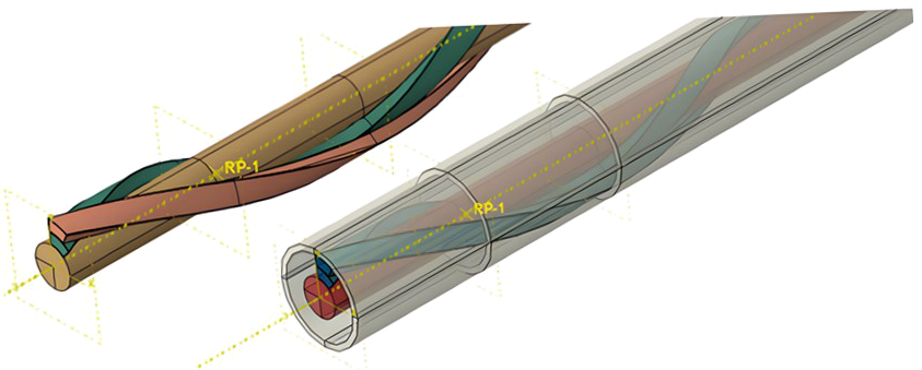
The cable assembly was built as a master parametric model in which the helix equations (1)–(3) drive a family of sweep features — one per strength-member layer — sharing the same four independent parameters (R, p, d, N) per layer. Because 2D drawings referenced these features directly (full model–drawing associativity), a change to a single parameter propagated automatically through every affected view, section and dimension, removing the need to manually redraft views after a design change.
Multiple cable constructions (different diameters, layer counts and lay lengths) were managed as configurations/family-table instances of the same master geometry rather than as separate models, so a correction made once to the master sweep logic benefited every variant simultaneously. Sub-assemblies (core, each armor layer, jacket) were then combined under top-level assembly constraints that encoded the physical stacking condition — each layer’s pitch circle radius set equal to the sum of the underlying layer radius and strand diameter — so that interference was flagged automatically if an incompatible parameter set was entered.
Documentation
Drawings followed ISO 128 general presentation principles, ISO 1101 for geometric tolerancing, and ISO 2768 general tolerances for non-critical dimensions, with first-angle projection used throughout to match the site’s manufacturing drawing standard. Because the strand geometry is helical, a developed (flattened) view was required to specify the raw-material cut length ordered for each strength-member layer. This was obtained analytically rather than measured off the model: the arc length of one full turn of the helix is
and, since an axial cable span of length ℓ corresponds to ℓ/p full turns, the total developed strand length simplifies — using the lay-angle relation of Equation (2) — to a single, practical formula:
This relation was placed directly on the manufacturing drawing as a driving note next to the cut-length dimension, so that any future change to the lay angle automatically flagged a corresponding review of the ordered strand length — closing the loop between the geometric model of Section 2.1 and a real procurement quantity.
Results & outcomes
Because every drawing view referenced the same equation-driven master model, typical dimensional update cycles that previously required manual redrafting over roughly two to three days were completed the same day the design change was decided. A single parametric master shared across configurations removed duplicate geometry maintenance across the cable construction range, and pre-release verification against the worst-case and RSS stack-up models of Equations (7)–(8) caught two potential layer-clearance conflicts before they reached prototype build, contributing to a clean first-pass fit on subsequent hardware. The completed drawing package was released into Windchill PLM under formal change control (ECR/ECN workflow, structured BOM, revision history), giving manufacturing and quality a single authoritative source for every released dimension and tolerance.
Technical environment & standards
Modeling and drafting were carried out in Creo Parametric, using equation-driven curves and relations, family tables for configuration management, and native associativity to 2D drawings; SolidWorks was used for ancillary parts and quick geometric studies. All released data was managed in Windchill PLM (structured BOM, ECR/ECN change process, revision and access control). Drawings applied ISO 128 (general drawing principles), ISO 1101 (geometrical product specification / GD&T) and ISO 2768 (general tolerances for dimensions without an individual tolerance indication), with tolerance grades assigned using the ISO 286 standard tolerance unit of Equation (6).
Nomenclature
| Symbol | Meaning |
|---|---|
| R | Pitch radius of a strand layer |
| p | Lay length (axial advance per full helix turn) |
| α | Lay angle, measured from the cable axis |
| N | Number of strands in a layer |
| d | Strand diameter |
| t | Helix winding-angle parameter |
| ℓ | Cable span length along the cable axis |
| Lstrand | Developed (cut) strand length over span ℓ |
| D | Nominal feature diameter (ISO 286) |
| i | ISO 286 standard tolerance unit |
| Ti | Individual tolerance contribution in a dimension stack |
| TΣ | Combined (stacked) tolerance |
| Teff | Effective positional tolerance including MMC bonus |
| wi, sij, Sj | Criterion weight, candidate score and weighted total in the CAD-platform selection |
References
- ISO 128–series, Technical drawings — General principles of presentation, International Organization for Standardization.
- ISO 1101:2017, Geometrical product specifications (GPS) — Geometrical tolerancing, International Organization for Standardization.
- ISO 286–1:2010, ISO code system for tolerances on linear sizes, International Organization for Standardization.
- ISO 2768–1, General tolerances — Tolerances for linear and angular dimensions without individual tolerance indications, International Organization for Standardization.